ScribblingsOnGraph

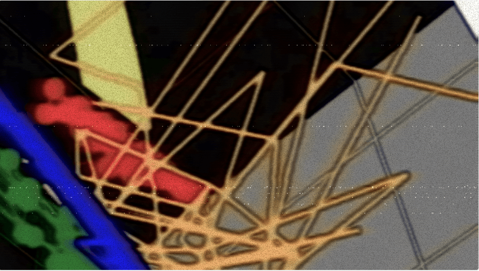
For this week's Creative Code challenge by @sableRaph: “Childhood Art”, ScribblingsOnGraph takes a 3D Graph in Python & coded audio in LiveCodeLab to show the childhood artform of scribbles and doodles.

Poem

Scribbling
Doodling the points that are Dabbling
Scribbling away the information
Seeing what they amass as a depiction

Video

Code

Python

import plotly.graph_objects as go
import numpy as np

import pandas as pd

#dataframe to make the scribbles
df = pd.read_csv("https://docs.google.com/spreadsheets/d/e/2PACX-1vQJPPryw-mxzKXzwhdhccm0fBQx4xGIt-mVbPRtUPADrhJRB9YKpFe7F9I2JZgNuM14a7-q9YVqIlwG/pub?gid=1407936083&single=true&output=csv")

# Create a Figure object
fig = go.Figure()

# Add the first trace
fig.add_trace(go.Scatter3d(
    x= df['Total CMYK'],y= df['diff(RGB-CMYK)'],z = df['X'],
    mode='lines',
    line=dict(color='blue', width=9),
    name='Scribble 1'
))

# Add the second trace
fig.add_trace(go.Scatter3d(
     x= df['Total CMYK'],y= df['Total RGB'],z = df['Total RGB'],
    mode='lines+markers',
    line=dict(color='red', width=5),
    name='Scribble 2'
))

# Add the third trace
fig.add_trace(go.Scatter3d(
     x= df['Mangeta'],y= df['diff(RGB-CMYK)'],z = df['Saturation2'],
    mode='lines+markers',
    line=dict(color='green', width=3),
    name='Scribble 3'
))

# Add the fourth trace
fig.add_trace(go.Scatter3d(
     x= df['Calories Per Cup'],y= df['Total RGB'],z = df['Total CMYK'],
    mode='lines',
    line=dict(color='orange', width=7),
    name='Scribble 4'
))

fig.add_trace(go.Mesh3d(x= df['Total CMYK'] * 2,y= df['Total RGB'] - 150,z = df['Total RGB'] + 100,opacity=1,color = 'yellow', name = 'Wall'
                  ))


fig.update_layout(
    scene = dict(
        xaxis = dict(nticks=4, range=[-300,800],backgroundcolor="black",gridcolor="white"),
                     yaxis = dict(nticks=4, range=[-200,800],backgroundcolor="grey",gridcolor="red"),
                     zaxis = dict(nticks=4, range=[-200,800],backgroundcolor="black",gridcolor="gold"),),
    width=700,
    margin=dict(r=20, l=10, b=10, t=10))

# Show the plot
fig.show()

LiveCodeLab

play "pianoLHChord" + int(random 2) ,'x------x-----'
play 'alienBeep'  ,'--x- ---- --x- -x-----x'
play 'tranceKick'  ,'-x-x ---x x--x- --xx'
play "crash" + int(random 13) ,'x--x-x'
play "hoover" + int(random 12) ,'x-x'
play "beep" + int(random 14) ,'xx--'
play "glass"  ,'x-x---x- -xx-x'
bpm 66